Single cell view plugin

The SingleCellView plugin can be used to run CellML models which consists of either a system of ordinary differential equations (ODEs) or differential algebraic equations (DAEs). The system may be non-linear.

Open a CellML file

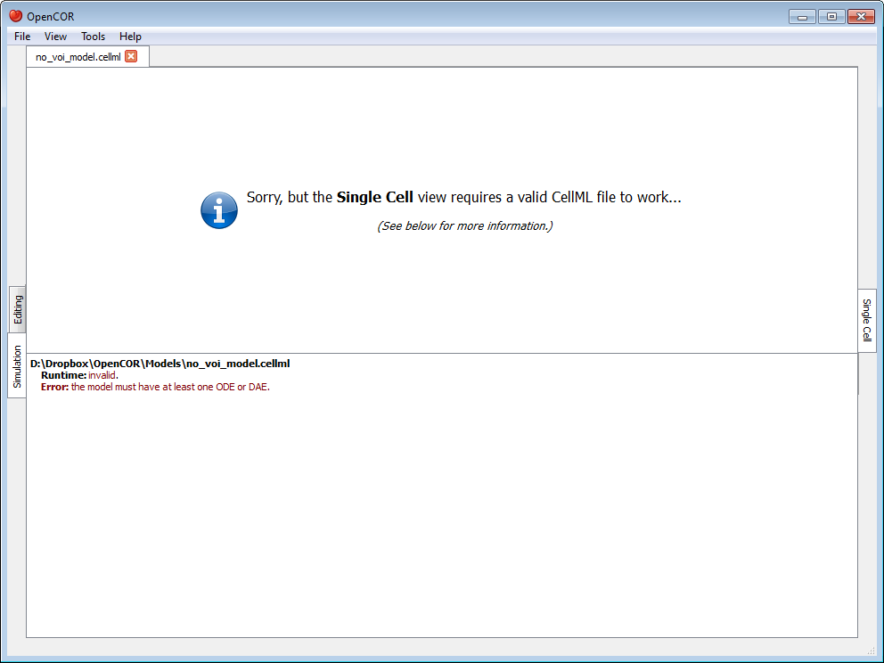
Upon opening a CellML file, OpenCOR will check that it can be used for simulation. If it cannot, then a message will describe the issue:

Alternatively, if the CellML file is valid, then the view will look as follows:

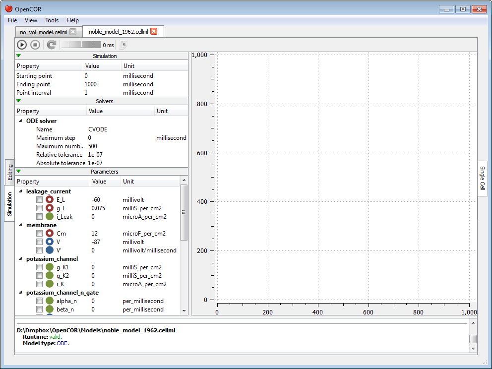
The view consists of two main parts, the first of which allows you to customise the simulation, the solver and the model parameters. The second part is used to plot simulation data. In the parameters section, each model parameter has an icon associated with it to highlight its type:

	(Editable) constant
	Computed constant
	(Editable) state
	Rate
	Algebraic

Simulate an ODE model

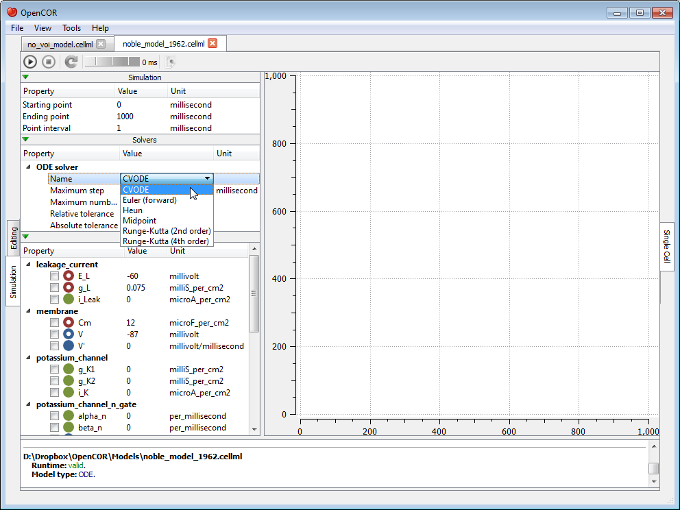
To simulate a model, you need to provide some information about the simulation itself, i.e. its starting point, ending point and point interval. Then, you need to specify the solver that you want to use. The solvers available to you will depend on which solver plugins you selected, as well as on the type of your model (i.e. ODE or DAE). In the present case, we are dealing with an ODE model and all the solver plugins are selected, so OpenCOR offers CVODE, forward Euler, Heun, Midpoint, and second- and fourth-order Runge-Kutta as possible solvers for our model.

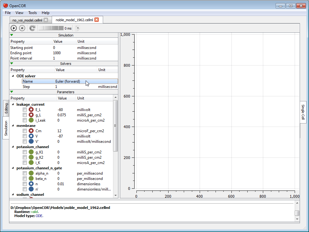
Each solver comes with its own set of properties which you can customise. For example, if we select Euler (forward) as our solver, then we can customise its Step property:

At this stage, we can run our model by pressing the F9 key or by clicking on the button. Then, or before, we can decide on a model parameter to be plotted against the variable of integration (which, here, is time since the simulation properties are expressed in milliseconds). All the model parameters are listed to the left of the view, grouped by components in which they were originally defined. To select a model parameter, click on its corresponding check box:

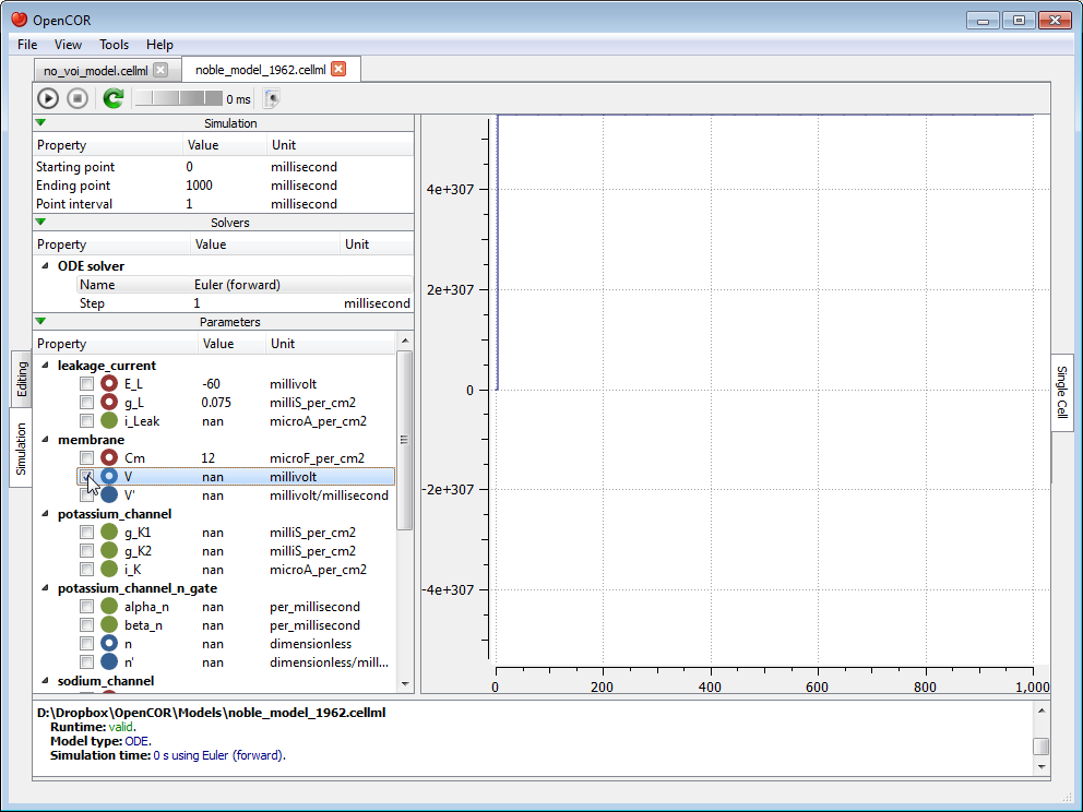
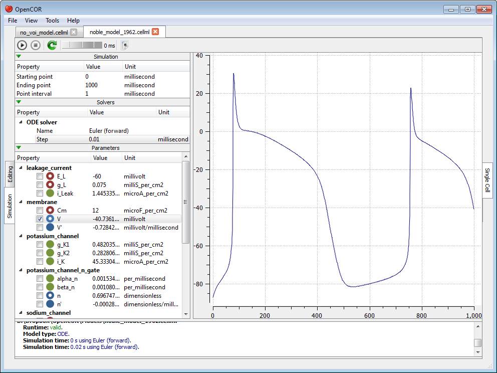
As can be seen, the simulation failed. Several model parameters, including the one we selected, have a nan value (i.e. not a number). In this case, it is because the solver was not properly set up. Its Step property is too big. If we set it to 0.01 milliseconds, reset the model parameters (by clicking on the button), and restart the simulation, then we get the following trace:

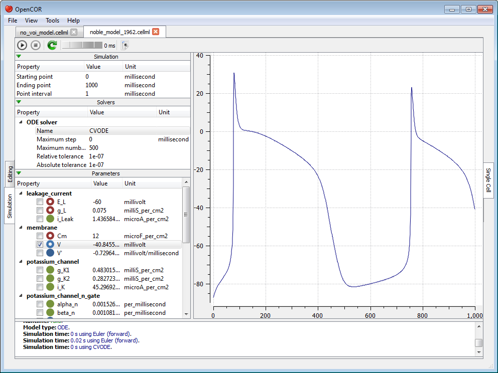
The (roughly) same trace can also be obtained using CVODE as our solver:

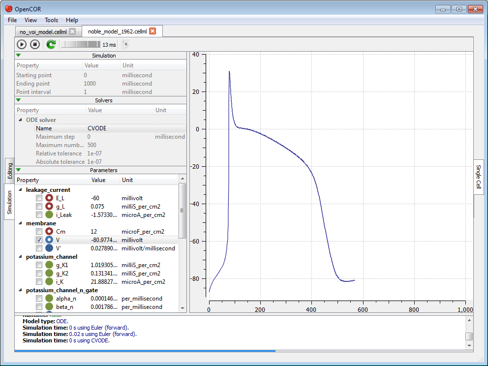
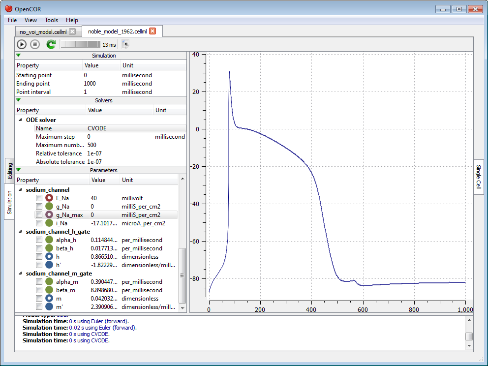
However, the simulation is so quick to run that we do not get a chance to see the progress of the simulation. Between the and buttons, there is a wheel which we can use to add a short delay between the output of two data points. Here, we set the delay to 13 ms. This allows us to rerun the simulation, after having reset the model parameters, and pause it at a point of interest:

Now, we can modify any of the model parameters identified by either the or icon, but let us just modify g_Na_max (under the sodium_channel component) by setting its value to 0 milliS_per_cm2. Then, we resume the simulation and we can see the effect on the model:

If we want, we could export all the simulation data to a comma-separated values (CSV) file. To do so, we need to click on the button.

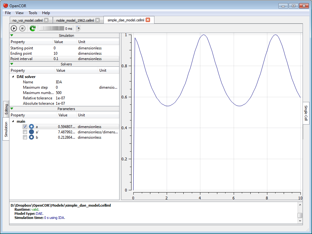
Simulate a DAE model

To simulate a DAE model is similar to simulating an ODE model, except that OpenCOR only offers one DAE solver (IDA) at this stage:

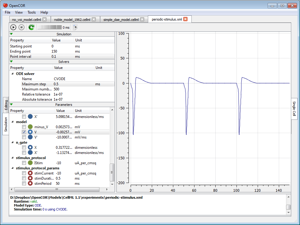
Simulate a CellML 1.1 model

So far, we have only simulated CellML 1.0 models, but we can also simulate CellML 1.1 models, i.e. models which import units and/or components from other models:

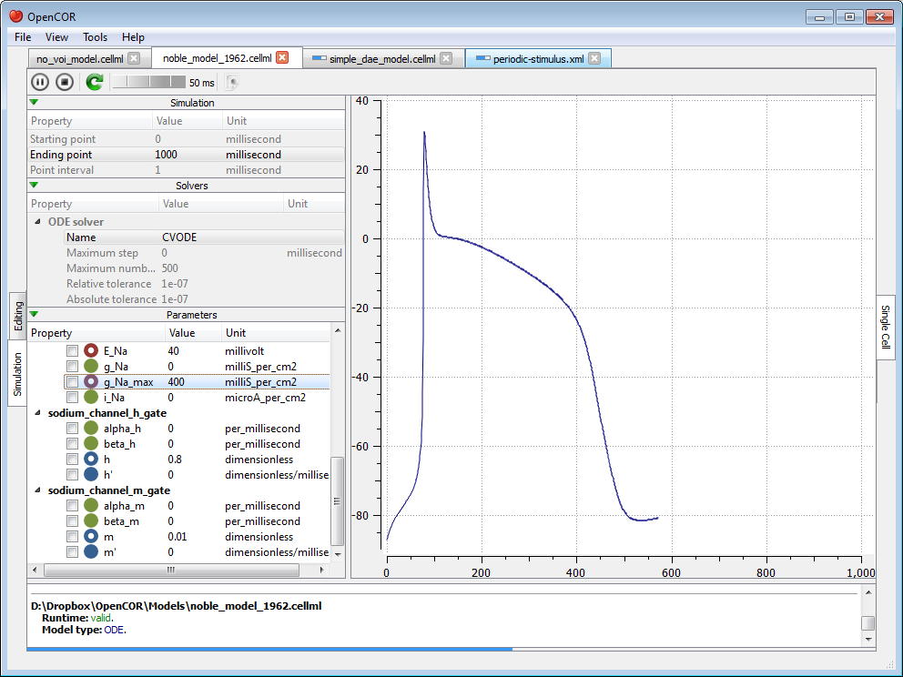
Simulate several models at the same time

Each simulation is run in its own thread which means that several simulations can be run at the same time. Simulations running in the 'background' display a small progress bar in the top tab bar while the 'foreground' simulation uses the main progress bar at the bottom of the view:

Plotting area

The plotting area offers several features which can be activated by:

• Zooming in:

  • holding the right mouse button down, and moving the mouse to the right/bottom to zoom in on the X/Y axis; or
  • moving the mouse wheel up.

• Zooming out:

  • holding the right mouse button down, and moving the mouse to the left/top to zoom out on the X/Y axis; or
  • moving the mouse wheel down.

• Zooming into a region of interest:

  • pressing Ctrl and holding the right mouse button down, and moving the mouse around.

• Panning:

  • holding the left mouse button down, and moving the mouse around (this obviously requires the plotting area to having been zoomed in in the first place).

• Coordinates of any point:

  • pressing Shift and holding the left mouse button down, and moving the mouse around.

• Copying the contents of the plotting area to the clipboard:

  • double-clicking the left mouse button.

Tool bar

	Run the simulation
	Pause the simulation
	Stop the simulation
	Reset all the model parameters
	Export the simulation data to CSV